2. Preprocessing temporally explicit data
Source:vignettes/V2_Preprocessing.Rmd
V2_Preprocessing.RmdSummary
- Overview
- Aligning rasters
- Spatiotemporal rarefaction
- Temporally explicit extraction
- Scaling rasters
- Spatiotemporal partitioning
- Generating pseudoabsences
- Outputs ready for modeling
Overview
The preprocessing phase of TemporalModelR takes raw occurrence records and environmental rasters and produces the structured inputs that the modeling functions expect. Six functions cover this phase, and they are typically run in order:
-
raster_align()- reproject and mask all rasters to a common reference grid. -
spatiotemporal_rarefaction()- subset occurrence points to one per pixel per time step. -
temporally_explicit_extraction()- extract environmental values matched to each point’s observation time. -
scale_rasters()- z-score rasters using the per-variable means and SDs from extraction. This step is optional, but should be applied for models sensitive to consistent scaling in predictor variables. If not, raw values and aligned rasters may be used. -
spatiotemporal_partition()- assign points to single fold, spatial, temporal, spatiotemporal, or random cross-validation folds. -
generate_absences()- produce fold-stratified pseudoabsences for presence/absence models.
This vignette walks through each step using the bundled synthetic
dataset described in the About
the Example Dataset vignette. Read that vignette first if you have
not already, as it explains the structure of the raw rasters and
occurrence points used here. We use the seasonal (compound
time-step) workflow throughout, with forest_cover
(annual), prseas (year-season), and elevation
(static) as predictors. The annual workflow is identical apart from
substituting pr_ann for prseas and dropping
season from the time columns.
library(TemporalModelR)
library(terra)
#> terra 1.9.34
library(sf)
#> Linking to GEOS 3.12.1, GDAL 3.8.4, PROJ 9.4.0; sf_use_s2() is TRUE

raw_dir  <- system.file("extdata/rasters_raw", package = "TemporalModelR")

pts_file <- system.file("extdata/points/synthetic_occurrence_points.csv",
                        package = "TemporalModelR")

ref_file <- file.path(raw_dir, "elevation.tif")
study_crs <- sf::st_crs(terra::rast(ref_file))
Aligning rasters
raster_align() standardizes every raster in a directory
to a single reference grid by reprojecting, resampling, and masking.
This is essential because downstream functions assume all environmental
layers share identical CRS, resolution, and extent. Even small
differences are enough to misalign extraction at the pixel level. With
the bundled dataset the raw rasters are already on the same grid, but we
run the alignment step to show the call pattern.
aligned_dir <- file.path(tempdir(), "rasters_aligned")

raster_align(
  input_dir        = raw_dir,
  output_dir       = aligned_dir,
  reference_raster = ref_file,
  resample_method  = "bilinear",
  overwrite        = TRUE
)
resample_method = "bilinear" is appropriate for
continuous variables like elevation and precipitation. Use
"near" for categorical rasters such as land cover classes;
bilinear interpolation between class codes would incorrectly generate
codes that do not exist.
We now have a directory of aligned rasters which can be used in downstream analyses.
aligned_dir <- system.file("extdata/rasters_aligned", package = "TemporalModelR")

list.files(aligned_dir, pattern = "\\.tif$")[1:6]
#> [1] "elevation_Masked_Updated.tif"       "forest_cover_1_Masked_Updated.tif"
#> [3] "forest_cover_10_Masked_Updated.tif" "forest_cover_11_Masked_Updated.tif"
#> [5] "forest_cover_12_Masked_Updated.tif" "forest_cover_13_Masked_Updated.tif"
Spatiotemporal rarefaction
spatiotemporal_rarefaction() reduces sampling bias and
pseudoreplication by retaining one occurrence per pixel per unique
time-step combination. The produces an only spatially rarefied table
(one point per pixel, regardless of time), and when
time_cols is provided, it additionally produces a
spatiotemporally rarefied table that preserves multiple observations
from the same pixel when they fall in different time steps.
This distinction matters for temporally explicit modeling. A static workflow would discard the second observation at the same pixel as redundant. A temporally explicit workflow keeps it, correctly recognizing that the environment at that pixel may have changed between the two observation times, making the second record carry unique information about the species’ niche.
rare_dir <- file.path(tempdir(), "rarefied")

rare_out <- spatiotemporal_rarefaction(
  points_sp        = pts_file,
  output_dir       = rare_dir,
  reference_raster = ref_file,
  time_cols        = c("year", "season"),
  xcol             = "x",
  ycol             = "y",
  points_crs       = study_crs,
  output_prefix    = "Pts_seasonal",
  verbose          = FALSE
)

rare_out$input_points
#> [1] 150

rare_out$spatial_points
#> [1] 84

rare_out$spatiotemporal_points
#> [1] 150
The spatial-only count is the number of unique pixels containing at least one record, retaining only 84 points of the starting 150. The spatiotemporal count is the number of unique pixel-year-season combinations and so will typically be larger whenever the dataset contains repeat visits to the same pixel in different time steps. In this instance, all 150 starting points contain unique pixel-year-season combinations.
Two CSVs are written to output_dir. The spatiotemporal
one is what we pass forward; the spatial-only file is retained for
reference and for users who want a static comparison:
rare_out$files_created
#> $spatiotemporal
#> [1] "/tmp/Rtmpy5e6TB/rarefied/Pts_seasonal_OnePerPixPerTimeStep.csv"
#>
#> $spatial
#> [1] "/tmp/Rtmpy5e6TB/rarefied/Pts_seasonal_OnePerPix.csv"
If we wanted to focus on annual variation rather than both annual and seasonal variation, we could instead run this focusing only ‘year’ as our time_col of interest. This would instead save all unique pixel-year combinations, but assume locations from the same year and location but different seasons share no new data.
rare_dir <- file.path(tempdir(), "rarefied")

rare_out_annual <- spatiotemporal_rarefaction(
  points_sp        = pts_file,
  output_dir       = rare_dir,
  reference_raster = ref_file,
  time_cols        = "year",
  xcol             = "x",
  ycol             = "y",
  points_crs       = study_crs,
  output_prefix    = "Pts_ann",
  verbose          = FALSE
)

rare_out_annual$input_points
#> [1] 150

rare_out_annual$spatial_points
#> [1] 84

rare_out_annual$spatiotemporal_points
#> [1] 144
This still retains many more points (144) than just the spatially explicit extraction.
Temporally explicit extraction
temporally_explicit_extraction() temporally aligns the
raster dataset with the temporal columns of the now rarefied species
occurrence dataset. For each occurrence record it extracts environmental
values from the raster matched to that point’s observation
time, rather than from a long-term average. The pairing between
point and raster is driven by variable_patterns: clean
variable names on the left, filename patterns with time placeholders on
the right.
ext_dir <- file.path(tempdir(), "extracted")

ext_out <- temporally_explicit_extraction(
  points_sp           = rare_out$files_created$spatiotemporal,
  raster_dir          = aligned_dir,
  variable_patterns   = c(
    "elevation"    = "elevation",
    "forest_cover" = "forest_cover_YEAR",
    "prseas"       = "prseas_YEAR_SEASON"
  ),
  time_cols           = c("year", "season"),
  xcol                = "X",
  ycol                = "Y",
  points_crs          = study_crs,
  output_dir          = ext_dir,
  output_prefix       = "extracted_seasonal",
  save_raw            = TRUE,
  save_scaled         = TRUE,
  save_scaling_params = TRUE,
  verbose             = FALSE
)

head(ext_out$raw_values)
#>   year season pixel_id elevation forest_cover prseas   x    y
#> 1   11 Spring        5      1247        0.846    310 450 1450
#> 2    4 Autumn        5      1247        0.856    370 450 1450
#> 3    7 Autumn        5      1247        0.825    370 450 1450
#> 4   13 Spring        6      1290        0.844    364 550 1450
#> 5   15 Autumn        6      1290        0.809    370 550 1450
#> 6    5 Autumn        6      1290        0.903    340 550 1450
A few details worth highlighting:
-
"elevation" = "elevation"is a static pattern with no placeholder, so every record is matched to the singleelevation.tifraster. -
"forest_cover" = "forest_cover_YEAR"substitutes each record’syearvalue forYEAR, so a record where the year column has a value of 7 is matched to the rasterforest_cover_7.tif. -
"prseas" = "prseas_YEAR_SEASON"substitutes bothyearandseason, so a record where the year column is 3 and the season column = spring is matched to the rasterprseas_3_Spring.tif. - We could also include
"pr_ann" = "pr_ann_YEAR"to match with annual measures of precipitation.
The same call generates three outputs:
ext_out$files_created
#> $raw
#> [1] "/tmp/Rtmpy5e6TB/extracted/extracted_seasonal_Raw_Values.csv"
#>
#> $scaled
#> [1] "/tmp/Rtmpy5e6TB/extracted/extracted_seasonal_Scaled_Values.csv"
#>
#> $scaling_params
#> [1] "/tmp/Rtmpy5e6TB/extracted/extracted_seasonal_Scaling_Parameters.csv"
The raw values file is what models that don’t need scaling will consume. The scaled file applies a z-score per variable using the means and SDs computed across all records. The scaling parameters file records those means and SDs so the same transformation can be applied to the prediction rasters, if necessary.
ext_out$scaling_params
#>       variable         mean           sd
#> 1    elevation 1936.4933333 462.38550909
#> 2 forest_cover    0.8641333   0.04070431
#> 3       prseas  317.3533333  73.04610447
Z-scoring matters when an algorithm is sensitive to variable scale,
such as those that rely on Euclidean distances and will misbehave if one
variable’s units dwarf the others (e.g. Temperature running from -10 to
38 C compared to precipitation running from 0 to 3000 mm. Use the
scaling parameters CSV when running scale_rasters() so the
rasters and the extracted point data share the same transformation.
Scaling rasters
scale_rasters() z-scores every raster in a directory
using the per-variable means and SDs from extraction. The transformation
is (value - mean) / sd, applied pixel-wise.
scaled_dir <- file.path(tempdir(), "rasters_scaled")

scale_rasters(
  input_dir           = aligned_dir,
  output_dir          = scaled_dir,
  scaling_params_file = ext_out$files_created$scaling_params,
  variable_patterns   = c(
    "elevation"    = "elevation",
    "forest_cover" = "forest_cover_YEAR",
    "prseas"       = "prseas_YEAR_SEASON"
  ),
  time_cols           = c("year", "season"),
  overwrite           = TRUE,
  verbose             = FALSE
)
variable_patterns mirrors the extraction call. For each
variable in the scaling parameters file, every matching raster in
input_dir is z-scored with the same mean and SD, this
guarantees the rasters and the points share a consistent
transformation.
scaled_dir <- system.file("extdata/rasters_scaled", package = "TemporalModelR")

list.files(scaled_dir, pattern = "\\.tif$")[1:6]
#> [1] "elevation_Scaled.tif"       "forest_cover_1_Scaled.tif"
#> [3] "forest_cover_10_Scaled.tif" "forest_cover_11_Scaled.tif"
#> [5] "forest_cover_12_Scaled.tif" "forest_cover_13_Scaled.tif"
We now have a directory of scaled rasters which we’ll use for future analyses.
Spatiotemporal partitioning
spatiotemporal_partition() assigns each occurrence
record to a cross-validation fold which will be used to create training
and testing datasets to build and assess our temporally explicit models.
The function supports five modes:
- Single fold. All points used for both training and testing. No held-out validation. Useful for a final production model after cross validated quality has been established, or when sample sizes are too small for splitting.
- Random. Folds are random shuffles with no spatial or temporal structure. Useful as a naive baseline.
- Spatial-only. Recursive k-d tree bisection produces geographically distinct contiguous regions, one per fold. Use when you want to test geographic transferability and don’t have time structure to exploit.
- Temporal-only. Each fold spans the full study area but covers a distinct slice of the time series, defined by quantile-based breaks. Use to test temporal transferability.
-
Spatiotemporal. Combines the two:
n_spatial_foldsare geographically distinct folds andn_temporal_foldsare time-restricted folds. Tests both kinds of transferability simultaneously.
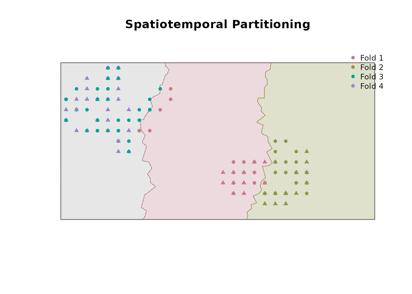
We use the spatiotemporal design with two folds in each pool. The
function requires the scaled (or raw) extracted points as input, a
polygon defining the study area, and a single time_cols
column (unlike the multi-column placeholders elsewhere; see
?spatiotemporal_partition for the rationale).
ext_scaled_file <- system.file(
  "extdata/points/extracted_seasonal_Scaled_Values.csv",
  package = "TemporalModelR"
)

study_area_sf <- sf::st_as_sf(sf::st_as_sfc(
  sf::st_bbox(c(xmin = 0, xmax = 3000, ymin = 0, ymax = 1500),
              crs = study_crs)
))

partition <- spatiotemporal_partition(
  reference_shapefile_path = study_area_sf,
  points_file_path         = ext_scaled_file,
  xcol                     = "x",
  ycol                     = "y",
  points_crs               = study_crs,
  time_cols                = "year",
  n_spatial_folds          = 2,
  n_temporal_folds         = 2,
  max_attempts = 10,
  max_imbalance = 0.15,
  create_plot              = TRUE,
  verbose                  = FALSE
)
partition$summary
#> parameter value
#> 1 total_folds 4
#> 2 n_spatial_folds 2
#> 3 n_temporal_folds 2
#> 4 n_balanced_folds 0
#> 5 n_random_folds 0
#> 6 partition_mode spatiotemporal
#> 7 total_points 150
#> 8 points_removed 0
#> 9 pct_rows_removed 0
#> 10 final_imbalance_pct 14.67
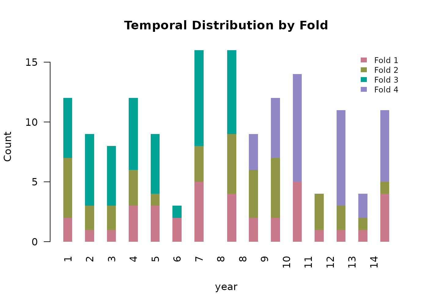
#> 11 temporal_partitioning_enabled TRUEThe returned points_sf carries a fold
column alongside the original predictor columns. Two of the four folds
are geographically restricted but span the full time series; the other
two overlap spatially and span the remainder of the study area but are
restricted to a distinct time slice each.
For partitioning purposes, time information must be encoded in a
single column based on what temporal scale is relevant for the desired
partitioning. Both example workflows in this package use the coarsest
time scale for partitioning time_cols = "year" at this step
(the season is preserved in the point data for later modeling and
prediction, just not used for fold construction). If both year and
season are conceptually meaningful for fold breaks, encode them into a
single ordered numeric column before partitioning. Alternatively,
partitioning could be done across seasons to view the environmental
transferability of seasonal environmental values.
Generating pseudoabsences
generate_absences() produces fold-stratified
pseudoabsence/background points for presence/absence modeling.
Pseudoabsences measure the environmental characteristics of locations
not otherwise characterized by species occurrences and are essential for
GLMs, GAMs, and random forests when no ‘true absence’ points exist. The
hypervolume method is presence-only and does not need them.
Four generation methods are supported:
- Random. Uniform sampling across the study area with a small buffer around presences to avoid exact overlap.
- Buffer. Sampling within a user-specified radius of presence locations. Useful when you want pseudoabsences from the same general environment as the presences, on the assumption that nearby unsampled locations are more likely to represent true absence than locations far from any survey effort.
-
Environmental. Cells outside the species’
environmental tolerance envelope are identified as candidates, then
k-means clustering selects a spatially representative subset. When
buffer_distanceis also supplied the environmental filtering is restricted to within that buffer, implementing the three-step approach of Senay et al. (2013). -
User data. A user-supplied set of points is used
directly as the absence locations rather than generating them.
Environmental values are extracted internally at each point’s matched
time step using the same
raster_dirandvariable_patternsas the other methods. Fold assignment is performed automatically by spatial join against the partition’s fold boundaries, with any points outside the spatial folds routed to temporal folds by their time value. This is the appropriate method when you have true absence records, or target-group background points from a separate survey.
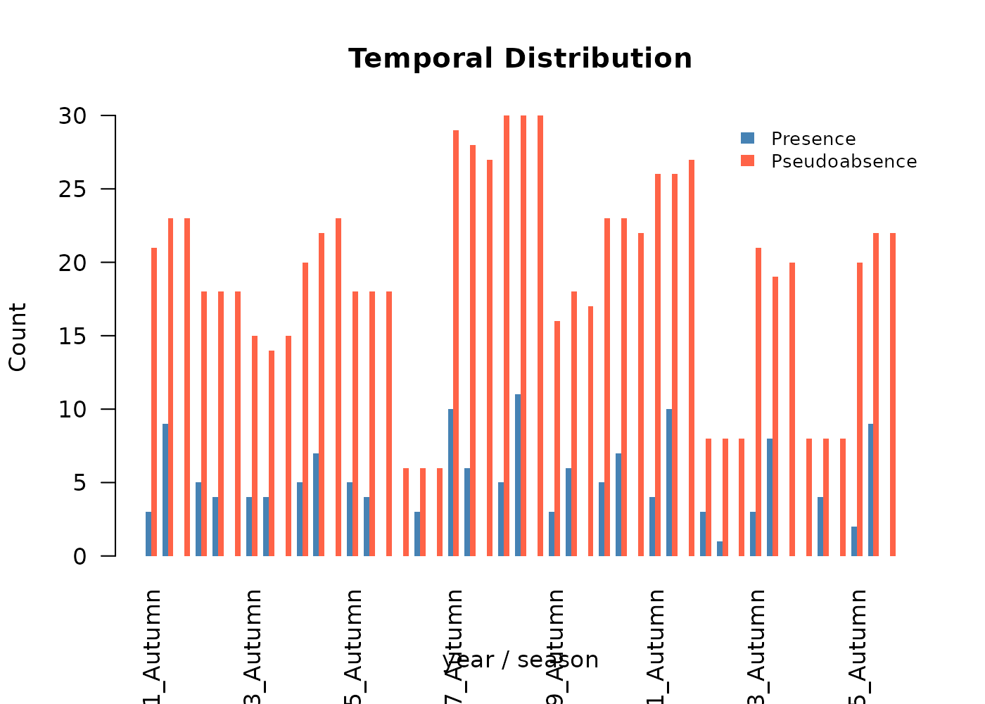
The function distributes pseudoabsences across folds and across time steps in proportion to the presences in each fold-time combination, so the potential environmental conditions experienced by each pseudoabsence match those experienced by the presences it complements.
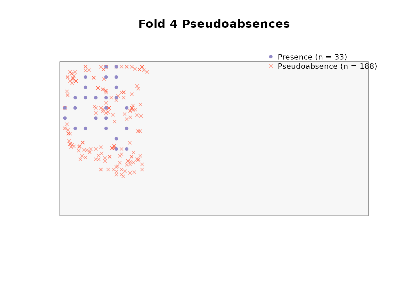
Buffer method
We use the buffer method with a 300 m radius (three pixels at the synthetic landscape’s 100 m resolution) and a 2:1 pseudoabsence-to-presence ratio:
absences <- generate_absences(
  partition_result         = partition,
  reference_shapefile_path = study_area_sf,
  raster_dir               = scaled_dir,
  variable_patterns        = c(
    "elevation"    = "elevation",
    "forest_cover" = "forest_cover_YEAR",
    "prseas"       = "prseas_YEAR_SEASON"
  ),
  method                   = "buffer",
  buffer_distance          = 300,
  ratio                    = 2,
  time_cols                = c("year", "season"),
  create_plot              = TRUE,
  plot_by_fold             = TRUE,
  verbose                  = FALSE
)
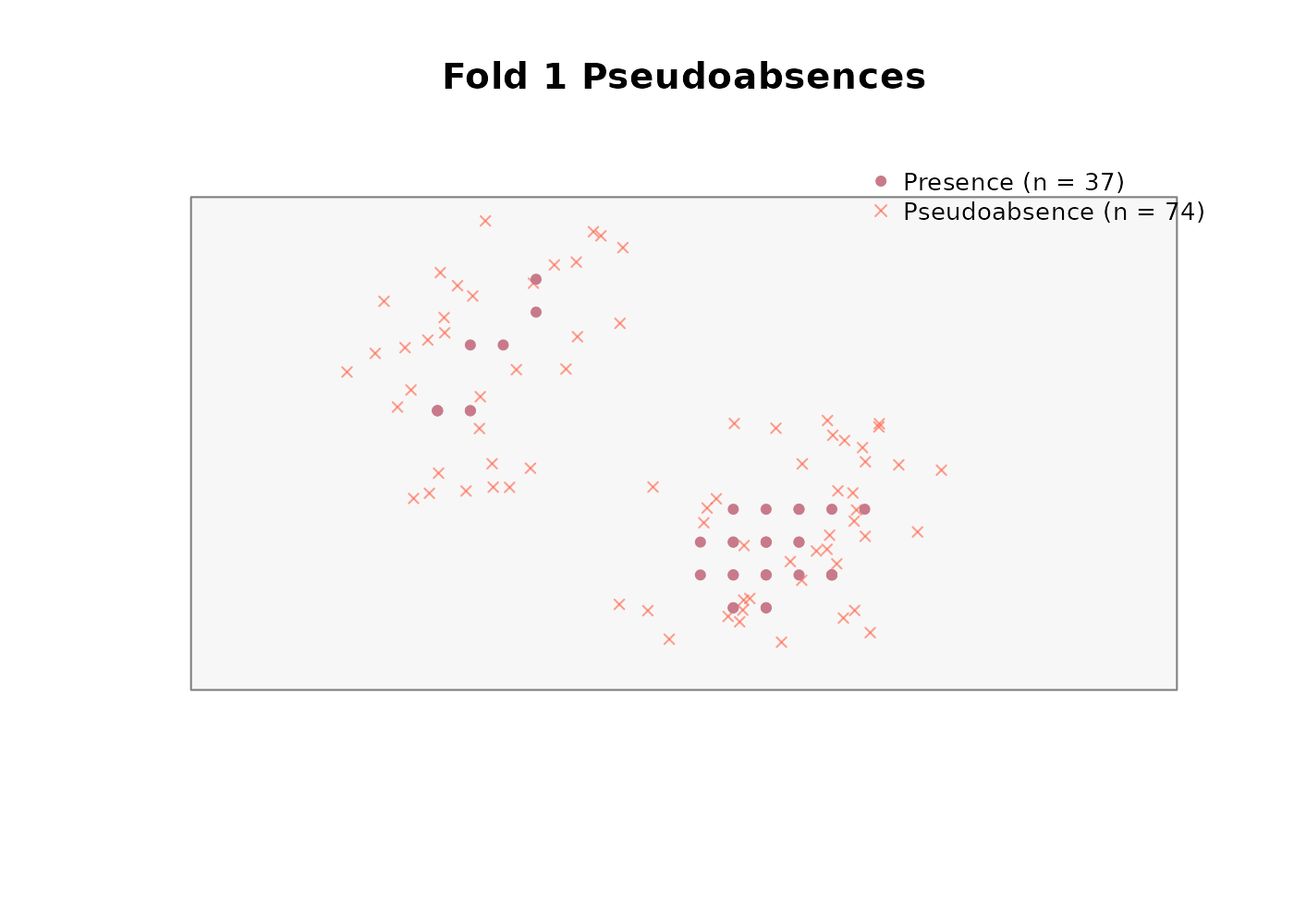
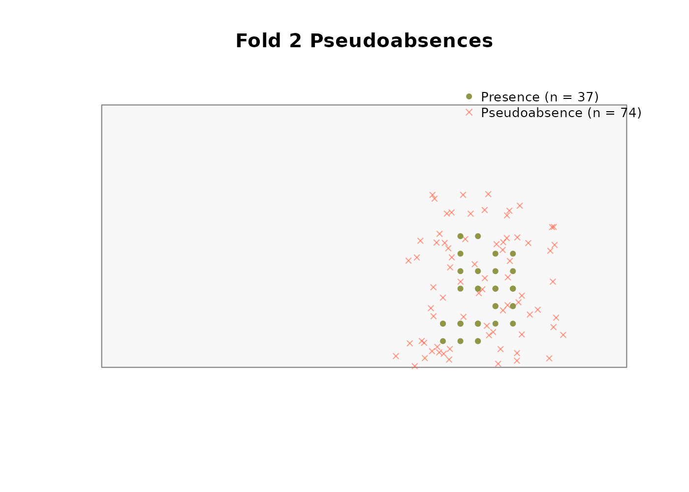
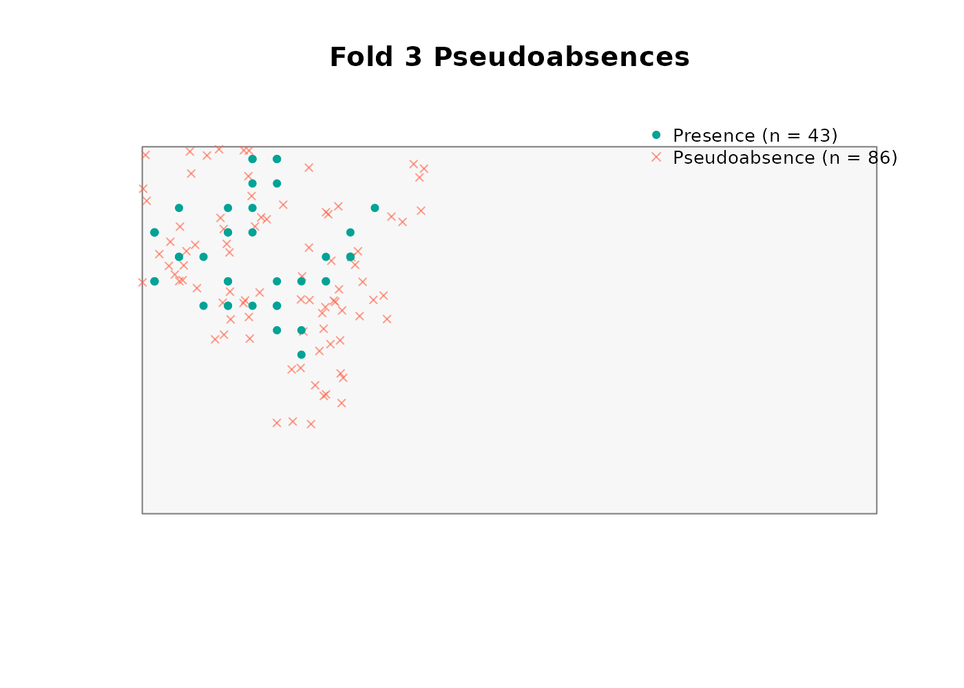
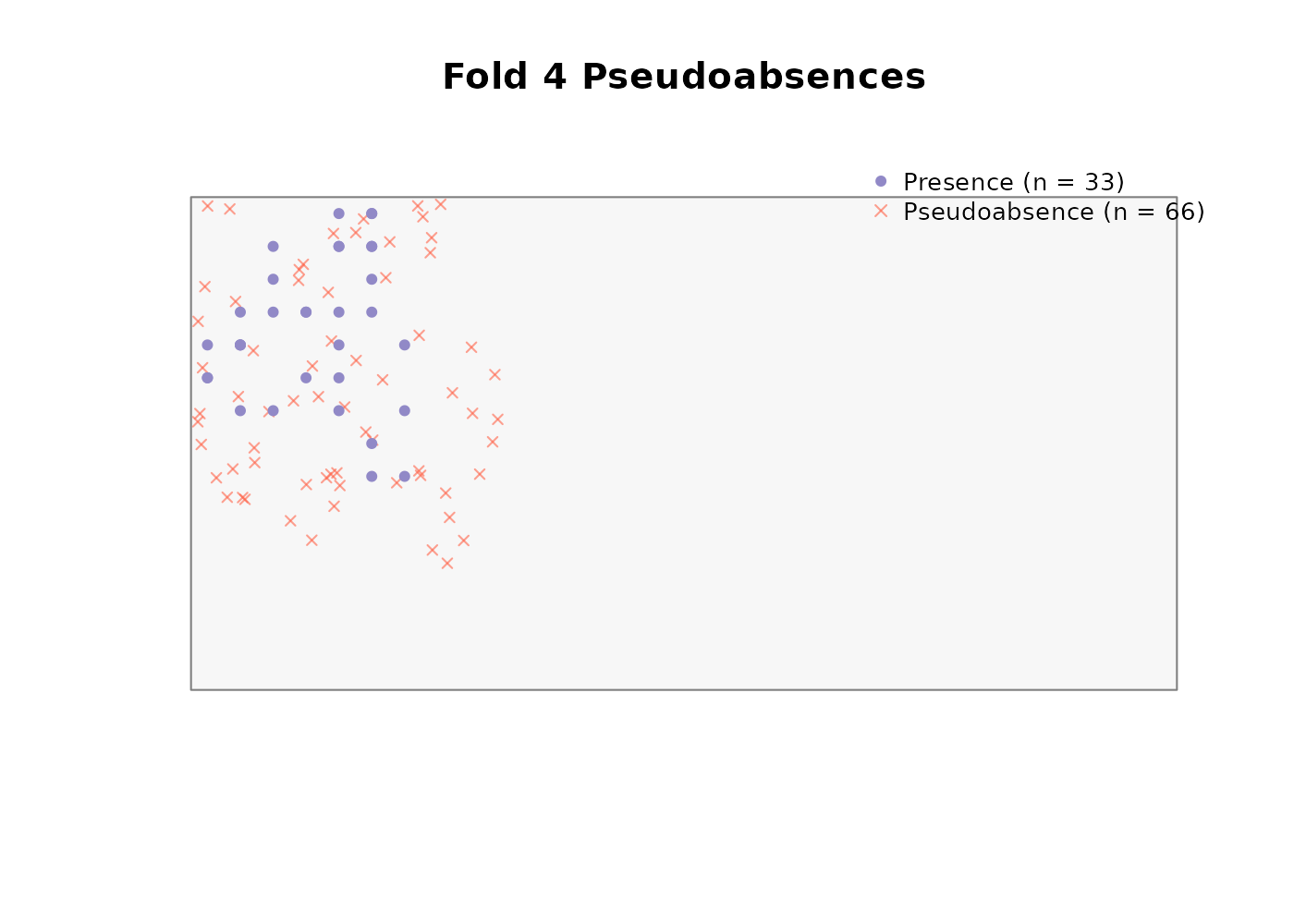
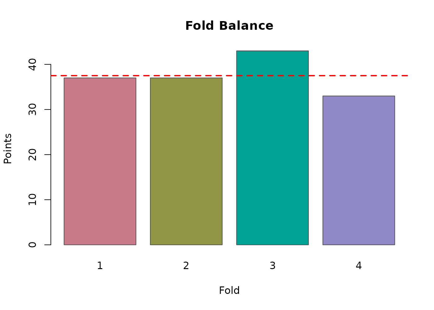
absences$summary
#> fold n_presences n_pseudoabsences ratio_achieved
#> 1 1 37 74 2
#> 2 2 37 74 2
#> 3 3 43 86 2
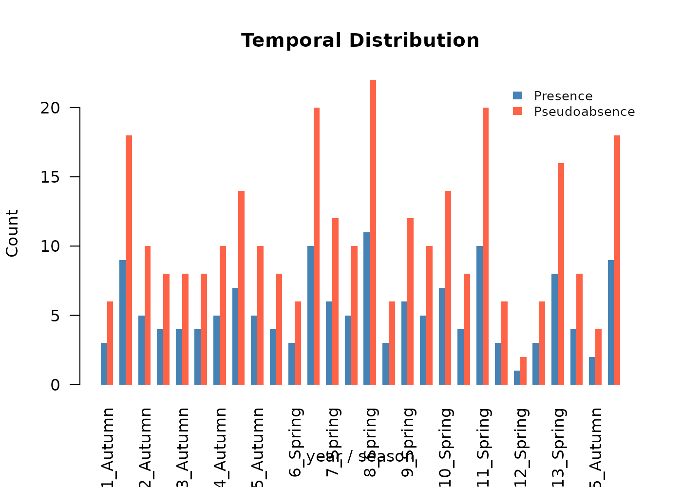
#> 4 4 33 66 2Note that variable_patterns and time_cols
here use both year and season. The
pseudoabsences are stamped with year-season values just like the
presences, and the environmental values attached to them are pulled from
the matching time-specific raster. This consistency is what keeps the
temporally explicit workflow intact through the model fitting step.
User data method
The generate_absences function alternatively allows for
users to process a set of defined absences for use with downstream
operations in this package. These points may represent true absence
records, such as negative occupancy survey locations, or may represent
pseudoabsence locations, such as occupancy locations for similar taxa
used as a proxy for survey effort. When using
method = "user_data", the function assigns each point to a
fold, then extracts temporally matched environmental values exactly as
it would for generated pseudoabsences. The output is identical except
for the fact that the points were not generated internally, and this
output can subsequently be used in any function requiring outputs from
generate_absences.
We consider synthetic_user_presences.csv as a second
related species to our species of interest. We assume that the survey
methodology is similar for both species, and any surveys conducted for
this second species would also have subsequently detected our species of
interest if it was present.
user_pts_file <- system.file(
  "extdata/points/synthetic_user_presences.csv",
  package = "TemporalModelR"
)

user_pts <- utils::read.csv(user_pts_file)

head(user_pts)
#>           x         y year season pres
#> 1 1115.2174 1241.3043    1 Spring    1
#> 2 1979.0323  566.1290    1 Spring    1
#> 3  814.0000  802.0000    1 Spring    1
#> 4 1514.5161  333.8710    1 Spring    1
#> 5 1747.0149  444.0299    2 Spring    1
#> 6  960.2041 1029.5918    2 Spring    1

nrow(user_pts)
#> [1] 900
The file has the same x, y,
year, season columns as the primary occurrence
data. Before passing it to generate_absences(), we apply
the same spatiotemporal rarefaction step used for the primary presences.
This ensures that if the second species’ dataset contains multiple
records in the same pixel and time step due to repeat surveys or
aggregated data, only one is retained, preventing pseudoreplication in
the absence set for the same reason it is prevented in the presence
set.
user_rare_dir <- file.path(tempdir(), "rarefied_user")

user_rare_out <- spatiotemporal_rarefaction(
  points_sp        = user_pts_file,
  output_dir       = user_rare_dir,
  reference_raster = ref_file,
  time_cols        = c("year", "season"),
  xcol             = "x",
  ycol             = "y",
  points_crs       = study_crs,
  output_prefix    = "Pts_user",
  verbose          = FALSE
)

user_rare_out$input_points
#> [1] 900

user_rare_out$spatiotemporal_points
#> [1] 846
We pass the rarefied file to generate_absences() via
user_absence_data, along with the coordinate column names
and CRS so that it can be processed as pseudoabsences for future
modeling.
absences_user <- generate_absences(
  partition_result         = partition,
  reference_shapefile_path = study_area_sf,
  raster_dir               = scaled_dir,
  variable_patterns        = c(
    "elevation"    = "elevation",
    "forest_cover" = "forest_cover_YEAR",
    "prseas"       = "prseas_YEAR_SEASON"
  ),
  method                   = "user_data",
  user_absence_data        = user_rare_out$files_created$spatiotemporal,
  xcol                     = "X",
  ycol                     = "Y",
  points_crs               = study_crs,
  time_cols                = c("year", "season"),
  create_plot              = TRUE,
  plot_by_fold             = TRUE,
  verbose                  = FALSE
)
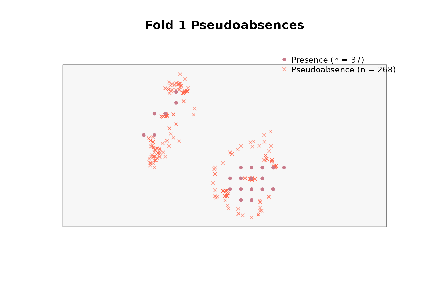
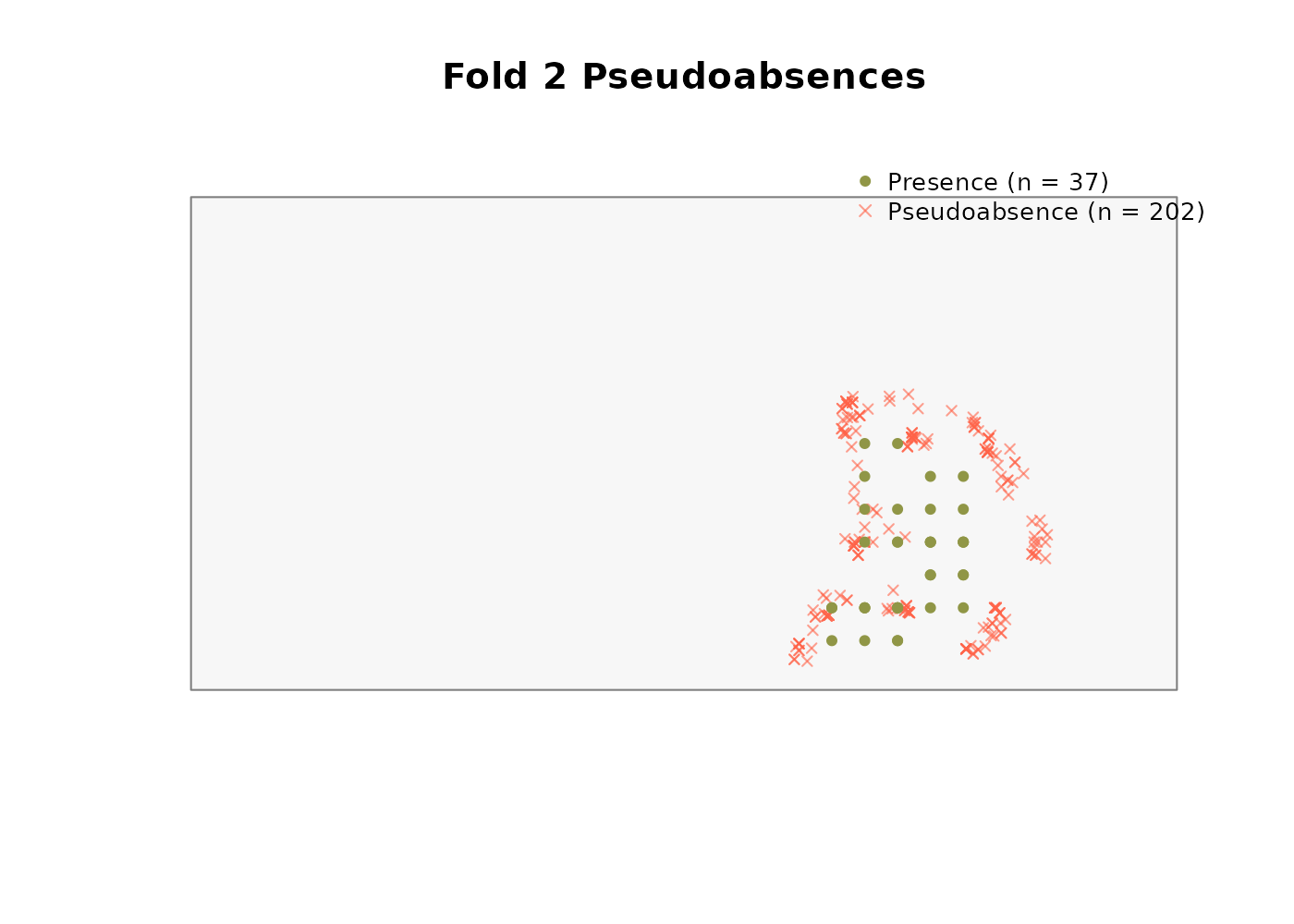
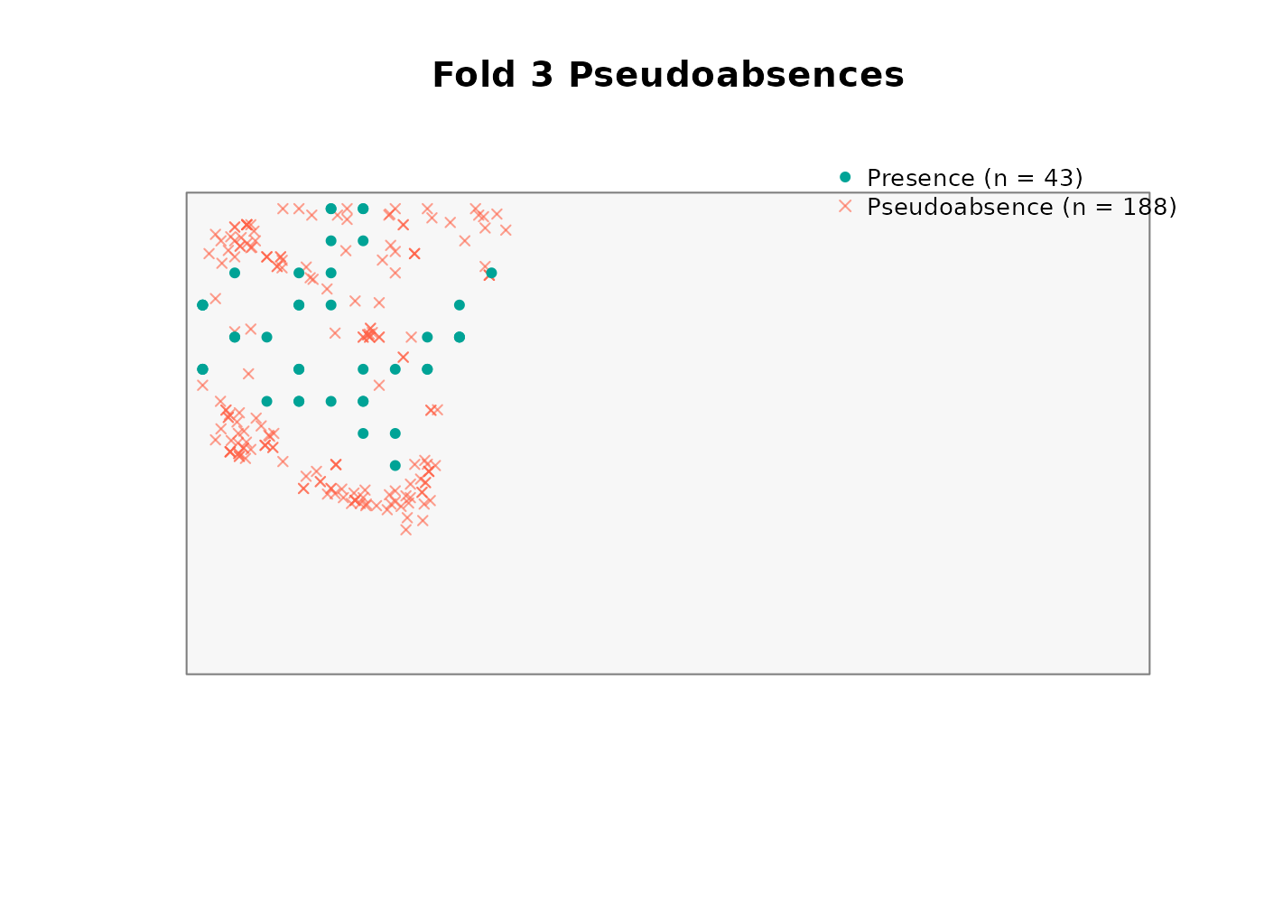
absences_user$summary
#>   fold n_presences n_pseudoabsences ratio_achieved
#> 1    1          37              268          7.243
#> 2    2          37              202          5.459
#> 3    3          43              188          4.372
#> 4    4          33              188          5.697
The result has the same structure as any other
generate_absences() output and can be passed directly to
any of the model builders.
Outputs ready for modeling
At this point the three key downstream inputs are in hand:
-
scaled_dir- the directory of scaled (or aligned inrasters_aligned, if scaling was skipped) rasters from which environmental conditions will be projected across space and time. -
partition- the rarefied, fold-assigned, time explicit environment data from species occurrence points. -
absences- the fold-stratified pseudoabsences with matching environmental attributes.
These are passed directly to any of the four model builders covered in the following parallel vignettes:
Once a model is fitted, predictions are projected through space and
time using generate_spatiotemporal_predictions(), and the
resulting prediction stack is summarized in the Post-processing
predictions vignette.